Assignment 3: Texture Synthesis
The purpose of this assignment is to implement and understand the texture synthesis approach of Efros and Leung.
Note. It is recommended to use Google Colab for this assignment, and it is required to use the matplotlib library version 3.8.0. In the given Jupyter Notebook file, you need to manually run pip install matplotlib==3.8.0; detailed instructions are provided in the notebook.
The assignment
-
First, you should make sure you understand the approach of Efros and Leung from the course notes and textbook. You should also read the original paper, “Texture Synthesis by Non-parametric Sampling” (PDF) published in 1999. You also may wish to visit Efros’ website that lists more recent research on this topic.
-
To simplify your task of implementing this method we have prepared some Python code that does the more difficult portions, so that you only have to fill in some of the basic matching routines. This code and the sample images are available in a zip file, hw3colab.zip. You should download this file to your directory and unzip it.
-
The zip file contains a sample image of a donkey in the file donkey.jpg. There is also an image showing the region to be filled (shown in black) and the sample texture region (shown as a white rectangle) in the file donkey2.jpg. There is a Jupyter Notebook file (named Assignment3.ipynb) which provides an interactive environemnt for executing this assignment.
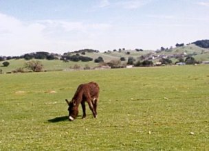
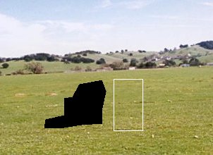
Original image Region to be texture filled You can open the file Assignment3.ipynb on Google Colab and follow the instructions. Make sure to copy all the contents of the zip file into the same directory where the notebook file is located. Please note that while you can use the notebook file for executing and showing the results, you need to add your code directly to the
Holefill.py, as instructed below.The
Holefill.pywill print two figures inline: one containing the orginal image and the other showing the region to be filled as well as the texture region. Once you run this line, you will be asked,Are you happy with this choice of fillRegion and textureIm?TypeYesto proceeed. Finally, the script should display an image, in which the empty space is filled with the new texture. As this skeleton program is missing some critical routines, the texture will initially be filled in as all black. -
(8 points)First, you need to complete the implementation of theComputeSSDfunction that computes the sum squared difference (SSD) between an image patch and the texture image, for each possible location of the patch within the texture image. It must ignore empty pixels that have a value of 1 in the given mask image. Skeleton code for this function is provided inHolefill.py.HINTS: The image patch is called
TODOPatch, and it is a square patch of size[2 * patchL + 1, 2 * patchL + 1, 3]. Note that the final dimension of 3 means that there are 3 colour values for each pixel. The texture image,textureIm, is of size[texImRows, texImCols, 3]. There is also a mask (an image of 1s and 0s) that specifies which elements inTODOPatchare empty and waiting to be filled in. The mask is calledTODOMaskand it contains a 1 for each empty pixel and a 0 for each pixel that has a useful value. Its first 2 dimensions are the same asTODOPatch, but it does not have the third dimension. You must ignore the empty pixels when computing the result. Note that the result,SSD, will have size[texImRows - 2 * patchL, texImCols - 2 * patchL]because it is only defined where the patch completely overlaps the texture. Further note that, as given inHolefill.py, theTODOPatchandtextureImarguments toComputeSSDhave data typeunit8. This is not a suitable data type for computing the required SSD. A simple Python trick to coerce a number to floating point is to multiply it by1.0. Do this, inComputeSSD, as needed. -
(6 points)The next section ofHolefill.pytakes the SSD image created above and chooses randomly amongst the best matching patches to decide which patch to paste into the texture image at that point. Next you need to complete the implementation of theCopyPatchfucntion which copies this selected patch into the final image. Remember again that you should only copy pixel values into the hole section of the image, and the existing pixel values should not be overwritten. Skeleton code forCopyPatchis provided inHolefill.py, along with comments explaining the arguments.Note that this technique of copying a whole patch is much faster than copying just the center pixel as suggested in the original Efros and Leung paper. However, the results are not quite as good. We are also ignoring the use of a Gaussian weighted window as described in their paper.
Hand in a printed copy of the donkey image after texture synthesis has been used to remove the donkey. Note that the texture synthesis might take some time to fill in all the empty spaces.
-
(5 points)Try running this texture synthesis method on some new images of your choosing. You will need to indicate the area of the removed region in the code. You can load your own image by altering the line that readsdonkey.jpginHolefill.py. You will need to select small regions to avoid long run times.In order to specify the custom fill and texture regions yourself, you can use the
polyselect.pyfile (Section 3 of the Jupyter Notebook file). To make it compatible with Jupyter Notebook, you need to installipymplusing the commands:pip install ipymplFollowing this you need to set the inline interaction operation using:
%matplotlib ipymplTo run it from notebook execute the following command:
%run polyselect.pyThe donkey image will be displayed. You draw a polygon by selecting each successive vertex with a left mouse click. To save the polygon, simply right click at any location on the image. To select the region to be filled type
0in the prompt. To select a texture region type1. To try an image other than the provided donkey image, you will have to alter the variableimnamearound line95. Regions you specify yourself will be saved for subsequent use as the filesfill_region.pklandtexture_region.pkl, overwriting existing files with the same name. Note: Be sure to save copies of the originalfill_region.pklandtexture_region.pklfiles.Hand in texture synthesis results for
2new images (different from the donkey image), where one shows the algorithm performing well and the other shows it performing poorly. For each example, show both the original image and the modified one. Briefly describe why the method failed in the case in which it performed poorly. -
(6 points)Take a look at the code inHolefill.pywhich randomly selects from the best matching patches. This takes an argumentrandomPatchSDwhich is the standard deviation of the number of the patch that gets chosen. If this value is set to0, then the optimal patch (minimum of the SSD image) is always chosen. If this value is large, then the patch choice will be more random. Experiment with this value and withpatchLwhich defines the size of the synthesis patches.Provide separate explanations for the effects of the
randomPatchSDandpatchLparameters. For each parameter, describe the expected results when the value is too small and when it is too large, and explain why these results occur.
Deliverables
Hand in your functions (i.e., *.py files), and the Jupyter Notebook Assignment3.ipynb. These must have sufficient comments for others to easily understand the code. You will lose marks for insufficient or unclear comments. In addition, submit the requested images and answers in a single PDF file. Specifically the PDF file should include the following:
- the donkey image after texture synthesis has been used to remove the donkey
- the texture synthesis examples for the 2 different images of your choosing. For each example, include both the original image and the modified one.
- the answers (discussions and/or explanations) to the questions
All deliverables should be submitted through Canvas.
© 2018 Leonid Sigal