Third edition of Artificial Intelligence: foundations of computational agents, Cambridge University Press, 2023 is now available (including the full text).
9.2 One-Off Decisions
Basic decision theory applied to intelligent agents relies on the following assumptions:
- Agents know what actions they can carry out.
- The effect of each action can be described as a probability distribution over outcomes.
- An agent's preferences are expressed by utilities of outcomes.
It is a consequence of Proposition 9.1 that, if agents only act for one step, a rational agent should choose an action with the highest expected utility.

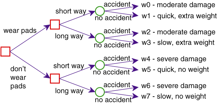
Thus, the robot has to decide whether to wear the pads and which way to go (the long way or the short way). What is not under its direct control is whether there is an accident, although this probability can be reduced by going the long way around. For each combination of the agent's choices and whether there is an accident, there is an outcome ranging from severe damage to arriving quickly without the extra weight of the pads.
To model one-off decision making, a decision variable can be used to model an agent's choice. A decision variable is like a random variable, with a domain, but it does not have an associated probability distribution. Instead, an agent gets to choose a value for a decision variable. A possible world specifies values for both random and decision variables, and for each combination of values to decision variables, there is a probability distribution over the random variables. That is, for each assignment of a value to each decision variable, the measures of the worlds that satisfy that assignment sum to 1. Conditional probabilities are only defined when a value for every decision variable is part of what is conditioned on.
Figure 9.4 shows a decision tree that depicts the different choices available to the agent and their outcomes. [These are different from the decision trees used for classification]. To read the decision tree, start at the root (on the left in this figure). From each node one of the branches can be followed. For the decision nodes, shown as squares, the agent gets to choose which branch to take. For each random node, shown as a circle, the agent does not get to choose which branch will be taken; rather there is a probability distribution over the branches from that node. Each path to a leaf corresponds to a world, shown as wi, which is the outcome that will be true if that path is followed.
What the agent should do depends on how important it is to arrive quickly, how much the pads' weight matters, how much it is worth to reduce the damage from severe to moderate, and the likelihood of an accident.
The proof of Proposition 9.1 specifies how to measure the desirability of the outcomes. Suppose we decide to have utilities in the range [0,100]. First, choose the best outcome, which would be w5, and give it a utility of 100. The worst outcome is w6, so assign it a utility of 0. For each of the other worlds, consider the lottery between w6 and w5. For example, w0 may have a utility of 35, meaning the agent is indifferent between w0 and [0.35 : w5, 0.65:w6], which is slightly better than w2, which may have a utility of 30. w1 may have a utility of 95, because it is only slightly worse than w5.
In a one-off decision, the agent chooses a value for each decision variable. This can be modeled by treating all the decision variables as a single composite decision variable. The domain of this decision variable is the cross product of the domains of the individual decision variables. Call the resulting composite decision variable D.
Each world ω specifies an assignment of a value to the decision variable D and an assignment of a value to each random variable.
A single decision is an assignment of a value to the decision variable. The expected utility of single decision D=di is
E(U|D=di) = ∑ω(D=di) U(ω)×P(ω),
where P(ω) is the probability of world ω, and
U(ω) is the value of the utility U in world
ω; ω  (D=di) means that the decision variable D has value di in world
ω. Thus, the expected-utility computation involves summing over the worlds that select the
appropriate decision.
An optimal single decision is the decision whose expected utility is maximal. That is, D=dmax is an optimal decision if
E(U|D=dmax)=maxdi∈dom(D)E(U|D=di),
where dom(D) is the domain of decision variable D. Thus,
dmax=argmaxdi∈dom(D)E(U|D=di).
= P(accident |wear_pads∧Which_way=short) ×utility(w0)
+(1-P(accident |wear_pads∧Which_way=short)) ×utility(w1),
where the worlds w0 and w1 are as in Figure 9.4, and wear_pads means Wear_Pads=true.


