Artificial
Intelligence

10.4.2 Learning to Coordinate

Due to the existence of multiple equilibria, in many cases it is not clear what an agent should actually do, even if it knows all of the outcomes for the game and the utilities of the agents. However, most real strategic encounters are much more difficult, because the agents do not know the outcomes or the utilities of the other agents.

An alternative to the deep strategic reasoning implied by computing the Nash equilibria is to try to learn what actions to perform. This is quite different from the standard setup for learning covered in Chapter 7, where an agent was learning about some unknown but fixed concept; here, an agent is learning to interact with other agents who are also learning.

This section presents a simple algorithm that can be used to iteratively improve an agent's policy. We assume that the agents are repeatedly playing the same game and are learning what to do based on how well they do. We assume that each agent is always playing a mixed strategy; the agent updates the probabilities of the actions based on the payoffs received. For simplicity, we assume a single state; the only thing that changes between times is the randomized policies of the other agents.

The algorithm PolicyImprovement of Figure 10.9 gives a controller for a learning agent. It maintains its current stochastic policy in the P array and an estimate of the payoff for each action in the Q array. The agent carries out an action based on its current policy and observes the action's payoff. It then updates its estimate of the value of that action and modifies its current strategy by increasing the probability of its best action.

In this algorithm, n is the number of actions (the number of elements of A). First, it initializes P randomly so that it is a probability distribution; Q is initialized arbitrarily to zero.

At each stage, the agent chooses an action a based on the current distribution P. It carries out the action a and observes the payoff it receives. It then updates its estimate of the payoff from doing a. It is doing gradient descent with learning rate α to minimize the error in its estimate of the payoff of action a. If the payoff is more than its previous estimate, it increases its estimate in proportion to the error. If the payoff is less than its estimate, it decreases its estimate.

It then computes a_best, which is the current best action according to its estimated Q-values. (Assume that, if there is more than one best action, one is chosen at random to be a_best.) It increases the probability of the best action by (n-1)δ and reduces the probability of the other actions by δ. The if condition on line 24 is there to ensure that the probabilities are all non-negative and sum to 1.

Even when P has some action with probability 0, it is useful to try that action occasionally to update its current value. In the following examples, we assume that the agent chooses a random action with probability 0.05 at each step and otherwise chooses each action according to the probability of that action in P.

An open-source Java applet that implements this learning controller is available from the book's web site.

If the other agents are playing a fixed strategy (even if it is a stochastic strategy), this algorithm converges to a best response to that strategy (as long as α and δ are small enough, and as long as the agent randomly tries all of the actions occasionally).

The following discussion assumes that all agents are using this learning controller.

If there is a unique Nash equilibrium in pure strategies, and all of the agents use this algorithm, they will converge to this equilibrium. Dominated strategies will have their probability set to zero. In Example 10.15, it will find the Nash equilibrium. Similarly for the prisoner's dilemma in Example 10.13, it will converge to the unique equilibrium where both agents take. Thus, this algorithm does not learn to cooperate, where cooperating agents will both give in the prisoner's dilemma to maximize their payoffs.

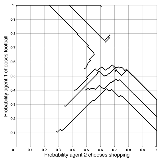
If there are multiple pure equilibria, this algorithm will converge to one of them. The agents thus learn to coordinate. In the football-shopping game of Example 10.12, it will converge to one of the equilibria of both shopping or both going to the football game. Which one it converges to depends on the initial strategies.

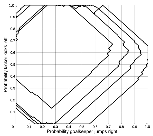
If there is only a randomized equilibrium, as in the penalty kick game of Example 10.9, this algorithm tends to cycle around the equilibrium.

Consider the two-agent competitive game where there is only a randomized Nash equilibrium. If an agent A is playing another agent, B, that is playing a Nash equilibrium, it does not matter which action in its support set is performed by agent A; they all have the same value to A. Thus, agent A will tend to wander off the equilibrium. Note that, when A deviates from the equilibrium strategy, the best response for agent B is to play deterministically. This algorithm, when used by agent B eventually, notices that A has deviated from the equilibrium and agent B changes its policy. Agent B will also deviate from the equilibrium. Then agent A can try to exploit this deviation. When they are both using this controller, each agents's deviation can be exploited, and they tend to cycle. There is nothing in this algorithm to keep the agents on a randomized equilibrium. One way to try to make agents not wander too far from an equilibrium is to adopt a win or learn fast (WoLF) strategy: when the agent is winning it takes small steps (δ is small), and when the agent is losing it takes larger steps (δ is increased). While it is winning, it tends to stay with the same policy, and while it is losing, it tries to move quickly to a better policy. To define winning, a simple strategy is for an agent to see whether it is doing better than the average payoff it has received so far.

Note that there is no perfect learning strategy. If an opposing agent knew the exact strategy (whether learning or not) agent A was using, and could predict what agent A would do, it could exploit that knowledge.