Discounted Least Squares (1997)
Discounted Least Squares Curve Fitting
- Blok (1997)
- Blok, H.(1997, 7/20). Retrieved from https://www.cs.ubc.ca/~rikblok/research/notes/discounted_least_squares/index.html
Version 1 — Rik Blok, 1997-07-20
1. Introduction
I recently wrote some code to make simple forecasts in a time series (a steadily accumulating set of \((x,y)\) data points). For its simplicity, I chose a least-squares fit to a straight line. The underlying behaviour of the system was continuously changing so it was unreasonable to expect the same parameters to be valid for all the data. As new data came in, I expected old data to become irrelevant, and I handled this by only fitting over the last \(N\) data points. Unfortunately, it became evident that this arbitrary parameter \(N\) I had chosen was very important to the fit, often producing pathological results: as \(N\) new data points were accumulated after an outlier (a strongly atypical \(y\)-value), it would suddenly be dropped from consideration and the forecast would undergo a discontinuous “jump”. I began to wonder if there was a way of steadily discounting the relevance of past data in a smoother and more natural way…
(Note: much of the text written here is a blatant copy from Press et al. ( Citation: 1992 Press, W., Teukolsky, S., Vetterling, W. & Flannery, B. (1992). Numerical Recipes in C: The Art of Scientific Computing (Second). Cambridge University Press. Retrieved from http://www.nr.com/ ) . They said it so well, I could not word it any better myself. In Chapter 16 they derive the least-squares technique I described above.)
2. Solution
We use the index \(i\) to label our data points where \(i=0\) indicates the most recently acquired data and \(i=1,2,3,\ldots\) indicate successively older data. Each data point consists of a triplet \((x,y,\sigma)\) where \(x\) is the independent variable (eg. time), \(y\) is the dependent variable, and \(\sigma\) is the associated measurement error in \(y\).
As new data arrives \((x_0,y_0,\sigma_0)\) we shift the indices of prior data to make room, and scale up the errors by some factor \(\gamma\in (0,1)\):
\[ (x_{i+1},y_{i+1},\sigma_{i+1})\leftarrow (x_i, y_i,\sigma_i/\gamma). \]If we define \(\sigma_i^*\) as the original value of \(\sigma_0\) then after applying \(i\) of the above operations
| \[ \sigma_i = \sigma_i^*/\gamma^i \] | (2.1) |
so, since \(\gamma<1\), the historical deviations grow exponentially as new information is acquired.
We wish to fit data to a model which is a linear combination of any \(M\) specified functions of \(x\). For example, the functions could be \(1,x,x^2,\ldots,x^{M-1}\), in which case their general linear combination,
\[ y(x) = a_1 + a_2 x + \cdots + a_M x^{M-1} \]is a polynomial of degree \(M-1\). The general form of this kind of model is
| \[ y(x) = \sum_{j=1}^M a_j X_j(x) \] | (2.2) |
where \(X_1(x),\ldots,X_M(x)\) are arbitrary fixed functions of \(x\), called the basis functions. Note that the functions \(X_j(x)\) can be wildly nonlinear functions of \(x\). In this discussion “linear” refers only to the model’s dependence on its parameters \(a_j\).
For these linear models we define a merit function
| \[ \chi^2 = \sum_{i=0}^N \left[ \frac{y_i - \sum_j a_j X_j(x_i)}{\sigma_i} \right]^2. \] | (2.3) |
We will pick as best parameters those that minimize \(\chi^2\). There are several different techniques for finding this minimum. We will focus on one: the singular value decomposition of the normal equations. To introduce it we need some notation.
Let \({\bf A}\) be a matrix whose \(N\times M\) components are constructed from the \(M\) basis functions evaluated at the \(N\) abscissas \(x_i\), and from the \(N\) measurement errors \(\sigma_i\), by the prescription
| \[ A_{ij} = \frac{X_j(x_i)}{\sigma_i}. \] | (2.4) |
The matrix \({\bf A}\) is called the design matrix of the fitting problem. Notice that in general \(\bf A\) has more rows than columns, \(N\geq M\), since there must be more data points than model parameters to be solved for.
Also define a vector \(\bf b\) of length \(N\) by
\[ b_i = \frac{y_i}{\sigma_i} \]and denote the \(M\) vector whose components are the parameters to be fitted, \(a_1,\ldots,a_M\), by \(\bf a\).
If we take the derivative of Eq. (2.3) with respect to all \(M\) parameters \(a_j\), we obtain \(M\) equations that must hold at the chi-square minimum,
| \[ 0 = \frac{1}{\sigma_i^2} \left[ y_i - \sum_j a_j X_j(x_i) \right] X_k(x_i)\;\; k=1,\ldots,M. \] | (2.5) |
Interchanging the order of summations, we can write Eq. (2.5) as the matrix equation
| \[ \sum_j \alpha_{kj} a_j = \beta_k \] | (2.6) |
where
| \[ \alpha_{kj} = \sum_i \frac{X_j(x_i) X_k(x_i)}{\sigma_i^2} \text{ or equivalently } [\alpha] = {\bf A}^T\cdot {\bf A} \] | (2.7) |
an \(M\times M\) matrix, and
| \[ \beta_k = \sum_i \frac{y_i X_k(x_i)}{\sigma_i^2} \text{ or equivalently } [\beta] = {\bf A}^T\cdot {\bf b} \] | (2.8) |
a vector of length \(M\).
Eq. (2.5) or (2.6) are called the normal equations of the least-squares problem. They can be solved for the vector parameters \(\bf a\) by singular value decomposition (SVD). SVD solves fixes many difficulties in the normal equations, including susceptibility to round-off errors. SVD can be significantly slower than other methods; however, its great advantage, that it (theoretically) cannot fail, more than makes up for the speed disadvantage. A good review of SVD techniques can be found in Press et al. ( Citation: 1992 Press, W., Teukolsky, S., Vetterling, W. & Flannery, B. (1992). Numerical Recipes in C: The Art of Scientific Computing (Second). Cambridge University Press. Retrieved from http://www.nr.com/ ) Section 2.6. In matrix form, the normal equations can be written as
| \[ [\alpha]\cdot {\bf a}=[\beta]. \] | (2.9) |
3. Covariance matrix
Let us define
| \[ [C] = [\alpha]^{-1}. \] | (3.1) |
Then
\[ {\bf a}=[C]\cdot [\beta] \text{ or } a_j = \sum_k C_{jk} \beta_k \]which allows us to determine \(\bf a\)’s dependence on the \(y_i\) values. From Eq. (2.7) we see that \([C]\) is independent of \(y_i\) so
| \[ a_j = \sum_j C_{jk} \sum_i A_{ik} \frac{y_i}{\sigma_i} \] | (3.2) |
and
\[ \frac{\partial a_j}{\partial y_i} = \sum_k C_{jk} \frac{A_{ik}}{\sigma_i}. \]The covariance between two parameters \(a_j\) and \(a_k\) is defined as
| \[ \begin{array}{rcl} \text{Covar}[a_j,a_k] & \equiv & \sum_i \sigma_i^2 \frac{\partial a_j}{\partial y_i} \frac{\partial a_k}{\partial y_i} \\ & = & \sum_i \sigma_i^2 \sum_{lm} C_{jl} \frac{A_{il}}{\sigma_i} \frac{A_{im}}{\sigma_i} \\ & = & \sum_{lm} C_{jl} C_{km} \alpha_{ml} \end{array} \] | (3.3) |
but since \([C]=[\alpha]^{-1}\) so
\[ \sum_m C_{km} \alpha_{ml} = \delta_{kl} \text{ or } [C][\alpha]={\bf 1} \]where \(\delta_{kl}\) is the Kronecker delta function. Hence Eq. (3.3) reduces to
| \[ \text{Covar}[a_j,a_k] = C_{jk} \] | (3.4) |
and we find that \([C]\) is the covariance matrix. The variance of a single parameter \(a_j\) is simply defined as
| \[ \text{Var}[a_j]=\text{Covar}[a_j,a_j]=C_{jj}. \] | (3.5) |
4. Storage and updating
So far we have made no mention of \(N\), the number of data points to be fit. As we will see an advantage of the discounted least squares method is that \(N\) becomes irrelevant. As data points are accumulated the oldest data becomes decreasingly relevant and eventually contribute negligibly to the fitting procedure. Hence we can theoretically apply this data to an infinite data set. But can this be practically implemented? The answer is…Yes!
Notice that as we acquire new data \((x_0,y_0,\sigma_0)\) according to Eq. (2.7) and (2.8) the matrix \([\alpha]\) and vector \([\beta]\) update as
| \[ \alpha_{kj} \leftarrow A_{0j} A_{0k} + \gamma^2 \alpha_{kj} = \frac{X_j(x_0) X_k(x_0)}{\sigma_0^2} + \gamma^2 \alpha_{kj} \] | (4.1) |
and
| \[ \beta_j \leftarrow A_{0j} b_0 + \gamma^2 \beta_j = \frac{X_j(x_0) y_0}{\sigma_0^2} + \gamma^2 \beta_j \] | (4.2) |
so it becomes clear that we need not even store the history of data points, but should rather store just \([\alpha]\) and \([\beta]\) and update them as new data is accumulated.
A useful measure we have neglected to calculate so far is \(\chi^2\),the chi-square statistic itself. In matrix notation Eq. (2.3) can be written
\[ \begin{array}{rcl} \chi^2 & = & ({\bf a}^T \cdot {\bf A}^T - {\bf b}^T) \cdot ({\bf A} \cdot {\bf a}-{\bf b}) \\ & = & {\bf a}^T \cdot {\bf A}^T \cdot {\bf A} \cdot {\bf a} - {\bf b}^T \cdot {\bf A} \cdot {\bf a} - {\bf a}^T \cdot {\bf A}^T \cdot {\bf b} + {\bf b}^T \cdot {\bf b} \\ & = & {\bf a}^T \cdot ([\alpha] \cdot {\bf a} - [\beta]) - [\beta]^T \cdot {\bf a} + {\bf b}^T \cdot {\bf b} \\ & = & {\bf b}^T \cdot {\bf b} - [\beta]^T \cdot {\bf a} \end{array} \]which appears to still depend on the data history in the first term. Let us define this term as a new variable \(\delta\),
\[ \delta \equiv {\bf b}^T \cdot {\bf b} = \sum_i b_i^2. \]Then, similarly to Eq. (4.1) and (4.2) \(\delta\) can be updated as more information is accumulated
| \[ \delta \leftarrow b_0^2 + \gamma^2 \delta = \frac{y_0^2}{\sigma_0^2} + \gamma^2 \delta. \] | (4.3) |
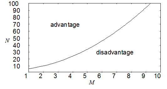
Figure 4.1: Discounted least-squares fitting has a computational storage advantage over traditional least-squares when \(N>M^2+M+4\) where \(N\) is the number of data points and \(M\) is the number of parameters to be fitted.
So, to store all relevant history information we need only remember \([\alpha]\), \([\beta]\), and \(\delta\) as well as the latest data triplet \((x_0,y_0,\sigma_0)\) for a total of \(M^2+M+4\) numbers, regardless of how many data points have been acquired. Figure 4.1 shows that for many practical problems discounted least-squares fitting requires less storage than other methods. Although it has not been tested, we expect a similar condition to hold for processing time because the number of calculations depend only on \(M\) instead of \(M\) and \(N\) as in traditional least-squares methods.
As the reader can justify, all of these values should be initialized (prior to any data) with null values: \([\alpha]={\bf 0}\), \([\beta]={\bf 0}\), and \(\delta=0\).
5. Memory, effective number of data points
For traditional least-squares fitting it is well known that if the measurement errors of \(y_i\) are distributed normally then the method is a maximum likelihood estimation and the expectation value (average) of Eq. (2.3) evaluates to
\[ \left\langle \chi^2 \right\rangle = N-M. \]This arises because \((y_i - y(x_i))/\sigma_i\) is distributed normally with mean 0 and variance 1, so the sum of \(N\) variances should equate to \(N\). The subtraction of \(M\) is necessary because \(M\) parameters can be adjusted to actually reduce the variances further. For instance, with \(N=M=1\) we can adjust the single parameter such that the curve passes precisely through the point \((x_0,y_0)\), with zero variance. Similarly, for our method
| \[ \begin{array}{rcl} \left\langle \chi^2 \right\rangle & = & \sum_{i=0}^\infty \gamma^{2 i} \left\langle \left[ \frac{y_i-y(x_i)}{\sigma_i^*}\right]^2 \right\rangle - M \\ & = & \sum_{i=0}^\infty \gamma^{2 i} - M \\ & = & \frac{1}{1-\gamma^2} - M \end{array} \] | (5.1) |
which strongly suggests an effective number of data points
| \[ N_{eff} \equiv \frac{1}{1-\gamma^2}. \] | (5.2) |
5.1. Memory
We now undertake a thought experiment to understand how \(N_{eff}\) comes into play. Consider a single parameter fit \(X(x_i)=1\) or \(y(x_i)=a\) to a long history of values \(y_i=1\) (regardless of \(x_i\)). Updating according to Eq. (4.1), (4.2), and (4.3) gives
\[ \begin{array}{rcr} \alpha & \leftarrow & 1 + \gamma^2 \alpha \\ \beta & \leftarrow & y + \gamma^2 \beta \\ \delta & \leftarrow & y^2 + \gamma^2 \delta \end{array} \]so after a long history of \(y=1\),
\[ \begin{array}{rl} \alpha & = 1 + \gamma^2 \left( 1 + \gamma^2(\cdots)\right) = 1 + \gamma^2 + \gamma^4 + \cdots \\ & = \frac{1}{1-\gamma^2} = \beta = \delta \end{array} \]which has a solution, in one dimension, of
\[ a = \frac{\beta}{\alpha} \]or \(y(x)=a=1\).
Now consider a sudden shift in the data stream to \(y_i=0\) (like a step function). How will this change our curve fit? The value of \(\alpha\) remains unchanged but \(\beta\) and \(a\) change as follows:
| \(y\) | \(\beta\) | \(a\) |
|---|---|---|
| \(\vdots\) | \(\vdots\) | \(\vdots\) |
| \(1\) | \(\alpha\) | \(1\) |
| \(0\) | \(\gamma^2 \alpha\) | \(\gamma^2\) |
| \(0\) | \(\gamma^4 \alpha\) | \(\gamma^4\) |
| \(\vdots\) | \(\vdots\) | \(\vdots\) |
Notice that \(a\) decays exponentially to the new equilibrium \(a=0\). The time constant \(\tau\) for the system (time for \(a\) to decay to \(1/e\)) is
\[ \begin{array}{l} \left( \gamma^2 \right)^\tau = e^{-1} \\ \Rightarrow \tau = \frac{-1}{2 \ln \gamma} \end{array} \]which is, as Figure 5.1 shows, almost identical to \(N_{eff}\) for all \(\gamma\).
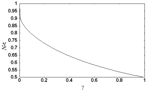
Figure 5.1: The difference between \(N_{eff}\) and \(\tau\) is strictly less than one. The main difference between the two is that \(\sigma_{N_{eff}} \rightarrow \infty \) as \(N_{eff}\rightarrow 1\) (as it should) while \(\sigma_\tau = \sqrt{e} \sigma_\tau^*\) for all \(\tau\). They converge as \(N_{eff}\rightarrow \infty\).
Thus, \(N_{eff}\) is indeed a practical measure of the effective number of data points in a fit. The fit is dominated by the most recent data \(i\leq N_{eff}\), and \(N_{eff}\) acts as the memory of the fitting procedure.
6. Unknown measurement errors
On occasion measurement uncertainties are unknown and least-squares fitting can be used to recover an estimate of these uncertainties. Be forewarned that this technique assumes normally distributed y data with identical variances. If this is not the case, the results become meaningless. It also precludes the use of a “goodness-of-fit” estimator (such as the incomplete gamma function, see Press et al. ( Citation: 1992 Press, W., Teukolsky, S., Vetterling, W. & Flannery, B. (1992). Numerical Recipes in C: The Art of Scientific Computing (Second). Cambridge University Press. Retrieved from http://www.nr.com/ ) Section 6.2) because it assumes a good fit.
We begin by assuming \(\sigma_i^*=1\) for all data points and proceeding with our calculations of \(\bf a\) and \(\chi^2\). If all (unknown) variances are equal \(\sigma^*=\sigma_i^*\) then Eq. (5.1) actually becomes
\[ \left\langle \chi^2 \right\rangle = (N_{eff} - M) \sigma^{*2} \]so the actual data variance should be
| \[ \sigma^{*2} = \frac{\chi^2}{N_{eff}-M}. \] | (6.1) |
We can update our parameter error estimates by recognizing that, from Eq. (3.2) and Eq. (2.4), the covariance matrix is proportional to the variance in the data, so
| \[ C_{jk} \leftarrow \frac{\chi^2}{N_{eff}-M} C_{jk}. \] | (6.2) |
7. Forecasting
Forecasting via curve fitting is a dangerous proposition because it requires extrapolating into a region beyond the scope of the data, where different rules may apply, and hence, different parameter values. Nevertheless, it often used simply for its convenience. We assume the latest parameter estimations apply at the forecasted point \(x\) and simply use Eq. (2.2) to predict \(y(x)\).
The uncertainty in the prediction can be estimated from the covariance matrix. The definition of variance for any distribution is the expectation value of the squared difference from the mean:
\[ \text{Var}[z] \equiv \left\langle \left( z - \langle z \rangle \right)^2 \right\rangle \]and the covariance between two variables is defined as
\[ \text{Covar}[z_1,z_2] \equiv \left\langle \left( z_1 - \langle z_1 \rangle \right) \left( z_2 - \langle z_2 \rangle \right) \right\rangle \]so Eq. (2.2) has a variance
\[ \begin{array}{rcl} \text{Var}[y(x)] & = & \text{Var}\left[ \sum_j a_j X_j(x) \right] \\ & = & \left\langle \left( \sum_j a_j X_j(x) - \sum_j \langle a_j \rangle X_j(x) \right) ^2 \right\rangle \\ & = & \sum_{jk} X_j(x) \left\langle \left( a_j - \langle a_j \rangle \right) \left( a_k - \langle a_k \rangle \right) \right\rangle X_k(x) \\ & = & \sum_{jk} X_j(x) \text{Covar}[a_j,a_k] X_k(x) \\ & = & X_j(x) C_{jk} X_k(x) \end{array} \]where \([C]\) is the covariance matrix discussed in Section 3 with possible updating, in the absence of measurement errors, according to Eq. (6.2).
The above gives the uncertainty in \(y(x)\), but in our derivation we have assumed the observed \(y\)-values were distributed normally around the curve where \(y(x)\) represents the mean of the distribution. Similarly for our prediction, \(y(x)\) is the prediction of the mean with its own uncertainty—-on top of which there is the measurement uncertainty of data around the mean. If the expected measurement uncertainty is given by \(\sigma'\) then the predicted observation \(y' \sim N(y(x),\sigma')\) or, with the substitution
\[ z' = y' - y(x) \]we assume \(z' \sim N(0,\sigma')\) regardless of the prediction \(y(x)\). In other words, \(z'\) and \(y(x)\) are mutually independent.
\[ \begin{array}{rcl} \text{Var}[y'] & = & \text{Var}[y(x) + z'] \\ & = & \left\langle \left( y(x) - \langle y(x) \rangle + z' - \langle z' \rangle \right)^2 \right\rangle \\ & = & \left\langle \left( y(x) - \langle y(x) \rangle \right)^2 + \left( z' - \langle z' \rangle \right)^2 + 2 \left( y(x) - \langle y(x) \rangle \right) \left( z' - \langle z' \rangle \right) \right\rangle \\ & = & \left\langle \left( y(x) - \langle y(x) \rangle \right)^2 \right\rangle + \left\langle \left( z' - \langle z' \rangle \right)^2 \right\rangle + 2 \left\langle \left( y(x) - \langle y(x) \rangle \right) \left( z' - \langle z' \rangle \right) \right\rangle \\ & = & \text{Var}[y(x)] + \text{Var}[z']. \end{array} \]The last step of dropping the covariance term is allowed because when two distributions are independent
\[ \left\langle \left( z_1 - \langle z_1 \rangle \right) \left( z_2 - \langle z_2 \rangle \right) \right\rangle = \left\langle z_1 - \langle z_1 \rangle \right\rangle \left\langle z_2 - \langle z_2 \rangle \right\rangle = 0 \]so our final results for the forecast \(y'\) at \(x\) are
| \[ \begin{array}{rcl} \langle y' \rangle & = & y(x) = \sum_j a_j X_j(x) \\ \text{Var}[y'] & = & \sum_{jk} X_j(x) C_{jk} X_k(x) + \sigma'^2. \end{array} \] | (7.1) |
If \(\sigma'\) is unknown it should be set to the same scale as historical measurement errors. If they are unknown, \(\sigma'\) should be estimated from Eq. (6.1).
8. Implementation
A sample implementation of the above method, using a polynomial fitting function is included in the DOS program dpolyfit.exe((Download {{:random_research:rik_s_notes:discounted_least_squares:dls.zip|dls.zip}} source code and executable, released to the public domain)). It is designed to make continuously updated parameter fits from data in the input stream, and output these parameters, or forecasts derived therefrom, to the output stream. It takes as a command-line parameter an initialization file containing preset parameters for the input format, fitting procedure, and output display. Common usages of this program are:
dpolyfit.exe inifile.ini <in.dat >out.dat
dpolyfit.exe inifile.ini <in.dat >>out.dat
Listing 8.1: Sample command-line parameters for program, where inifile.ini, in.dat, and out.dat are replaced with desired configuration, input and output files, respectively. The second version appends output to out.dat rather than overwriting it.
The behaviour of the program is controlled by the initialization file which contains the following options:
[Input]
Errors=No	; input s values?

[Fit]
Memory=14	; effective # data points, Neff in Eq. 5.2
Parameters=7	; # of parameters a to fit, M in Eq. 2.2

[Output]
Input=Yes	; print input (x,y,s) triplet to output?
Parameters=No	; print parameters a and errors to output?
Forecast=Yes	; print forecasted y to output?
Forecast Distance=0	; forecast y at x=x0+"Forecast Distance"

[Abort]	; end program when all of the following are true:
x=0
y=0
sig=0	; only compare s if "[Input] Errors=Yes"
Listing 8.2: Sample initialization file inifile.ini.
If “[Input] Errors=Yes” then the program expects three numbers per data point \((x_0,y_0,\sigma_0)\), each separated by white spaces (eg. “1.0 1.2 0.4”). Otherwise, only two are expected \((x_0,y_0)\).
The option “[Fit] Memory=...” contains \(N_{eff}\) as in Eq. (5.2). Generally, this must be strictly \(>0\), but if a negative number is entered it is interpreted as \(N_{eff}=\infty\), producing a traditional fit over all data points with no rescaling of the measurement errors.
If “[Output] Input=Yes” then the input values \((x_0,y_0,\sigma_0)\) are reproduced as the first three columns of the output file. Even if \(\sigma_0\) is unspecified, a best estimate is output, based on Eq. (6.1).
If “[Output] Parameters=Yes” then the next \(2 M\) columns of output are the parameters \(\bf a\) and their respective uncertainties, eg. “\(a_1 \delta a_1 \ldots a_M \delta a_M\)”.
If “[Output] Forecast=Yes” then the program generates another two columns of output. It calculates the forecast of \(y\) at \(x=x_0+\)"[Output] Forecast Distance" from Eq. (7.1) and prints out the forecasted \(y\) and its uncertainty.
The program ends when the input \((x_0,y_0,\sigma_0)\) or \((x_0,y_0)\) matches the values in “[Abort] x=... y=... sig=...” or “[Abort] x=... y=...”, respectively.
The design of this program might cause some confusion: even though the input data file is a complete set of data, the program only analyzes each data point successively, and all output is based on just this point and prior data. For example, forecasts are based only on past data, so by the end of the output file, all data points are considered but in the beginning results are based only on a single data point. The technique derived herein is better suited to time series with slowly accumulating data, rather than a complete data set on startup.
9. Summary
As in traditional least-squares methods, by differentiating the \(\chi^2\) merit function (Eq. (2.3)) of a linear model (Eq. (2.2)) we were able find a set of linear equations (Eq. (2.9)) which allowed us to solve for the optimal parameters which minimize \(\chi^2\). By scaling up the error tolerance of old data as new data is acquired (Eq. (2.1)) we were able to compact the information such that only an \(M \times M\) matrix \([\alpha]\) (Eq. (4.1)), an \(M\times 1\) vector \([\beta]\) (Eq. (4.2)), and a scalar \(\delta\) (Eq. (4.3)) need be stored to retain the full history of accumulated data. We found that the inverse of \([\alpha]\) (Eq. (3.1)) held the covariance matrix of the fitted parameters (Eq. (3.4) and (3.5)). We were able to compute a memory for this technique (Eq. (5.2)) which is comparable to the number of data points used in traditional least-squares fitting. By assuming a good fit we were able to estimate the measurement uncertainties if they were unknown, and apply this to reconstruct reasonable deviations in the fitted parameters (Eq. (6.2)). Finally, by extrapolating with the latest parameter estimates (assuming they were valid in the forecasted domain), we were able to make forecasts and estimate their uncertainties (Eq. (7.1)).
As my list of references will attest, I have done virtually no research to see whether the discounted least-squares method has already been discovered (as is undoubtedly the case) and what name it goes by. In deriving this, I did not care if I “reinvented the wheel” because my goal was to introduce myself to some of the statistical techniques, particularly those used in the derivation of uncertainties.
10. References
- Blok (1997)
- Blok, H.(1997, 7/20). Retrieved from https://www.cs.ubc.ca/~rikblok/research/notes/discounted_least_squares/index.html
- Press, Teukolsky, Vetterling & Flannery (1992)
- Press, W., Teukolsky, S., Vetterling, W. & Flannery, B. (1992). Numerical Recipes in C: The Art of Scientific Computing (Second). Cambridge University Press. Retrieved from http://www.nr.com/