Parallel Poisson (2004)
Updating in simulations of parallel Poisson processes
- Blok (2004)
- Blok, H.(2004, 10/15). Retrieved from https://www.cs.ubc.ca/~rikblok/research/notes/parallel_poisson/index.html
Version 1 — Rik Blok, 2004-10-15
Abstract
I explore how to efficiently implement Poisson processes in event-driven, multi-agent simulations. The most efficient strategy I am able to find uses a binary tree to implement the roulette wheel algorithm and results in \(O(\log_2 N)\) time to find the next event out of \(N\) total processes. These notes arose from discussions with Mario Pineda, Alistair Blachford, and Michael Doebeli. Unpublished.
1. Definition
— Rik Blok, 2004-09-26
A Poisson process is a sequence of random events where the probability of an event is constant per unit time. Usually it is described in terms of a sequence of multiple events but in this discussion I will focus on the occurrence of a single event in the sequence. Let \(c(t)\) be the cumulative probability that the event has occurred by time t (starting at \(t = 0\)). Then, by the definition of a Poisson process, the probability of the event occurring between \(t\) and \(t + dt\) is given by the p.d.f.
\[ p(t) dt = (1 − c)r dt \]where \(r\) is the average rate of the event sequence. This gives the probability that the event has not occurred yet \((1 − c)\) and then occurs in the specified interval \((r dt)\).
Since the p.d.f. is the derivative of the cumulative, \(p(t) \equiv dc/dt\), we find that
\[ \frac{dc}{1-c} = r\, dt \]so the cumulative distribution is given by
\[ c(t) = 1 - e^{-r t} \]and the p.d.f. is
\[ p(t) = r e^{-r t}. \]The above gives the distribution for a single event. Below, we expand this to consider a number of possible events, each given by a Poisson process with an unique rate \(r_j\) . The problem is: how do we simulate such a process efficiently?
2. Roulette wheel algorithm
— Rik Blok, 2004-10-01
In a discrete-event simulation it is possible to sample random deviates for all possible events and construct an event queue to determine the order or events but it is cumbersome. The roulette wheel algorithm is algorithmically simpler. Given rates \(r_j, j=1\ldots N\), the probability of event i acting first is
\[ \Pr(i\text{ first}) = \frac{r_i}{\sum_j r_j}. \]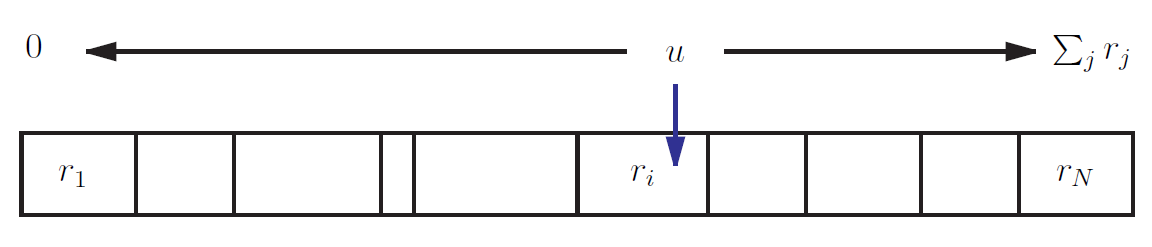
Figure 1: To select an event via the Roulette Wheel algorithm pick a random number \(u\) between \(0\) and \(\sum_j r_j\). Then it will land within the area delimited by \(r_i\) with probability \(r_i/\sum_j r_j\).
We can derive this from the Poisson distribution: let \(t_i\) be a random variable representing the waiting time to the first occurrence of event \(i\). Then the probability that event \(i\) is first (marginalizing over \(t_i\)) is
\[ \begin{array}{rcl} \Pr(t_i < \{t_j\}_{j\neq i}) & = & \int_0^\infty dt_i p_i(t_i) \prod_{j\neq i} (1 - c_j(t_i)) \\ & = & dt_i r_i e^{-\sum_j r_j t_i} \\ & = & \frac{r_i}{\sum_j r_j} \end{array} \]where \(p_i\) and \(c_i\) represent the distributions for event \(i\) with rate \(r_i\). As shown in Figure 1, to pick an event, just pick a uniform deviate \(0 \leq u < \sum_j r_j\), and select the maximum \(i\) such that
\[ \sum_{j\leq i} r_j \leq u. \]This method is simple to implement but computationally expensive since it requires \(O(N)\) operations (due to the summation) to compute each \(i\).
3. Rejection method
— Rik Blok, 2004-10-01
An alternative to the roulette wheel is the rejection method. The idea is to pick a random event \(i\) and sample whether it passes a trial. We will begin by determining what the probability of a successful trial, \(f\), should be. We would like the trial to be generic so that it only depends on the event rate, \(f(r_i)\). Given \(N\) processes, the probability of a single failed trial is
\[ \begin{array}{rcl} \Pr(\text{fail trial}) & = & \text{for any } j: \Pr(j)\, \Pr(\text{fail given }j) \\ & = & \sum_j \frac{1}{N} (1 − f(r_j)) \\ & = & 1 − \bar{f} \end{array} \]where \(\bar{f} = \sum_j f(r_j)/N\).
The probability of \(k\) failed trials followed by a successful \(i\) event is
\[ \Pr(k\text{ fails then }i) = \left[1 − \bar{f}\right]^k \frac{1}{N} f(r_i). \]So the probability of choosing \(i\) for any number \(k\) of failed trials is
\[ \begin{array}{rcl} \Pr(i\text{ first}) & = & \sum_{k \geq 0} \left[1 − \bar{f}\right]^k \frac{1}{N} f(r_i) \\ & = & \frac{f(r_i)}{N \bar{f}}. \end{array} \]Notice that this satisfies the normalization condition: \(\sum_i \Pr(i) = 1\).
What we’d like to find is a form for the trial probability \(f\) that produces the Poisson probability:
\[ \Pr(i\text{ first}) = \frac{r_i}{\sum_j r_j} = \frac{f(r_i)}{\sum_j f(r_j)}. \]Since this must hold independently of the rates \(r_j\) we must have \(f(r_j) \propto r_j\) which we can write as
\[ f(r) = \frac{r}{\hat{r}} \]for some constant \(\hat{r}\).
3.1. Efficient computation
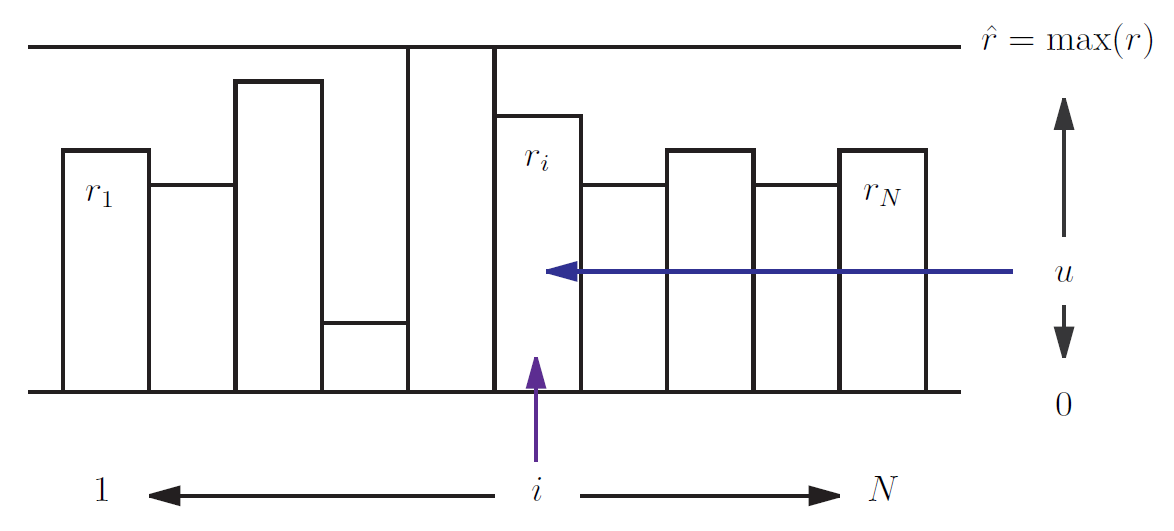
Figure 2: To select an event via the rejection method pick a random event \(i\) and a random deviate \(0 < u < \hat{r}\). Accept if \(u < r_i\) otherwise repeat.
We want to choose \(\hat{r}\) in order to minimize the computational cost of the rejection method. Recall that \(f\) is to be interpreted as a probability so it must obey \(f(r_j) \leq 1\) for all \(r_j\) which means that \(\hat{r} \geq \max(r_j)\). Each time a trial is failed more work is required for a new trial so the number of trials should be minimized. The probability of a single failed trial is \(1−\bar{r}/\hat{r}\) (where \(\bar{r} = \sum_j r_j/N\)) so the prob. of \(k\) trials is
\[ \begin{array}{rcl} \Pr(k\text{ trials}) & = & \text{for any }i:\Pr(k − 1\text{ fails then success with }i) \\ & = & \sum_i \left( 1 − \frac{\bar{r}}{\hat{r}}\right)^{k−1} \frac{1}{N} \frac{r_i}{\bar{r}} \\ & = & \left( 1 − \frac{\bar{r}}{\hat{r}}\right)^{k−1} \frac{\bar{r}}{\bar{r}} \end{array} \]and the expected number of trials is
| \[ \langle k \rangle = \sum_k k \Pr(k\text{ trials}) = \frac{\hat{r}}{\bar{r}}. \] | (1) |
So we can minimize \(\langle k \rangle\) by reducing \(\hat{r}\) as much as possible, ideally by choosing \(\hat{r} = \max(r_j)\). Then the actual number of trials \(\langle k \rangle\) depends on the distribution of rates. The best case is if \(\max(r_j) \propto \bar{r}\) so that \(\langle k \rangle = O(1)\) is independent of \(N\).
But if the rates are dynamic, if they change as the simulation progresses, then there is an added cost of continually updating \(\hat{r}\). The worst choice would be to check all \(N\) rates and reset \(\hat{r}\) appropriately whenever any rate changed. That would increase the cost of the rejection method to \(O(N)\) operations, no better than the Roulette Wheel.
An alternative would be to keep the rates sorted so that \(r_j \geq r_{j+1}\) for all \(j\). Then \(\hat{r} = r_1\), always. The cost involved would be that of adding and removing items from a sorted list. (I believe C++’s STL offers a ‘’(multi)map’’ container which is implemented as a binary tree giving typically \(O(\log N)\) cost. Hash tables may also be suitable.)
That was assuming \(\hat{r}/\bar{r}\) was independent of \(N\). More realistically, we might expect the highest rate in the set to scale as \(\hat{r} \propto \bar{r} \log N\) so the total computational expense of this approach would grow as \(O([\log N]^2)\) which is still much better than the Roulette Wheel.
4. Faster implementation by sampling two events?
— Rik Blok, 2004-10-05
I wonder if it is possible to find an even less costly method by sampling multiple event processes and comparing them? To explore this we will consider a variant of the rejection method where the trial probability of event \(i\) depends on a second sampled event \(j \neq i, f = f(r_i, r_j)\). If \(i\) is rejected then two new events are drawn. Is there a trial function \(f\) that reproduces the Poisson process?
Independent of \(j\) the probability of \(i\) passing any single trial is
\[ \Pr(i\text{ this trial}) = \frac{1}{N(N-1)} \sum_{j\neq i} f(r_i,r_j). \]The probability of failing a trial, independent of the event \(k\) chosen is
\[ \begin{array}{rcl} \Pr(\text{fail}) & = & \sum_k \Pr(\text{choose }k) \Pr(\text{fail given }k) \\ & = & \sum_{k,l\neq k} \frac{1}{N(N-1)} (1-f(r_k,r_l)) \\ & = & 1 - \bar{f} \end{array} \]where \(\bar{f} = \sum_{k,l}f(r_k,r_l)/N(N-1)\).
Like the rejection method, the probability of \(m\) failed trials then a successful event \(i\) is
\[ \Pr(m\text{ fails then }i) = \left[ 1-\bar{f} \right]^m \frac{1}{N(N-1)} \sum_{j\neq i} f(r_i,r_j) \]so the probability of event \(i\) occurring first is
\[\begin{array}{rcl} \Pr(i\text{ first}) & = & \sum_m \left[ 1-\bar{f} \right]^m \frac{1}{N(N-1)} \sum_{j\neq i} f(r_i,r_j) \\ & = & \frac{1}{\bar{f}} \sum_j \frac{f(r_i,r_j)}{N(N-1)}. \end{array} \]For this to produce Poisson updating we must have
\[ \frac{r_i}{\sum_k r_k} = \frac{\sum_j f(r_i,r_j)}{\sum_{k,l} f(r_k,r_l)} \]or \(r_k \propto \sum_{l\neq k} f(r_k,r_l)\) which means that we can write
\[ f(r_k,r_l) = r_k g(r_l) \]for some unknown function \(g\). Rather than working with \(g\) directly, it is more convenient to work with the partial sum \(G_i=\sum_{j\neq i} g(r_j)\) as we see here:
\[ \frac{r_i}{\sum_k r_k} = \frac{r_i \sum_{j\neq i} g(r_j)}{\sum_k r_k \sum_{l\neq k} g(r_l)} = \frac{r_i G_i}{\sum_k r_k G_k}. \]Recall, we are trying to detemine the form of \(G_i\) that reproduces Poisson updating. For arbitrary rates \(r_k\) the above equation reduces to \(\sum_k G_k = N G_i\) for all \(i\), which can only be satisfied if all \(G_i\) are equal. In other words, \(g(r) = \text{const.}\) independent of \(r\) so the second sampling is irrelevant and we fall back to the original rejection method. It appears there is no way to improve on the rejection method by sampling multiple events.
5. Rejection with adaptive correction
— Rik Blok, 2004-10-12
Mario came up with the idea of using the rejection method but relaxing restriction so that \(\hat{r} \geq \max(r)\) is not strictly maintained at exactly \(\max(r)\). It is cheap to enforce [with each new rate \(r_i\) just set \(\hat{r} = \max(\hat{r},r_i)\) which is \(O(1)\)] but has a hidden cost: wasted rejection trials if \(\hat{r}\) is too large. Mario’s idea was to recalculate \(\hat{r}\) if the failed trials \(k\) were ever found to exceed some arbitrary threshold \(k_\max\).
That’s good but I think we can do even better. There should be a way to choose how many //wasted// trials are acceptable. Recall from Eq. 1 that \(\langle k\rangle =\hat{r}/\bar{r}\). Since we can keep track of \(\bar{r}\) in constant \(O(1)\) time [if a rate changes from \(r_\text{old}\) to \(r_\text{new}\) then \(\bar{r} \gets \bar{r} + (r_\text{new} - r_\text{old})/N\) (where `\(\gets\)’ represents the assignment operator)] it is possible to compute the optimal expected number of trials per event whenever \(\max(r)\) is known,
| \[ k_\text{opt} = \frac{\max(r)}{\bar{r}}. \] | (2) |
Now we assume that \(k_\text{opt}\) remains roughly constant even as the rates change. Basically we’re assuming that \(\max(r) \propto \bar{r}\). So we only update \(k_\text{opt}\) occasionally, whenever we are sure of \(\max(r)\) (to be discussed).
Having a fairly accurate \(k_\text{opt}\) lets us estimate how many trials are being wasted because our value of \(\hat{r}\) is too high. It doesn’t tell us what \(\hat{r}\) should be, just when we’re spending too much effort in rejection trials. The goal then, is to determine a criterion for when it is more efficient to correct \(\hat{r}\) by reiterating the entire set of rates \(r_i\) instead of continuing to use our inefficient estimate.
The first thing we need to know is \(\omega\), the relative cost of one rejection trial versus one iteration of the correction loop:
\[ \omega = \frac{\text{cost(1 rejection trial)}}{\text{cost(1 correction loop)}}. \]This could be computed in advance and stored as a constant.
Then we keep track of the number of trials \(k_e\) actually required for every event \(e\). After \(E\) total events since the last correction the relative waste \(W\) on failed trials is approximately
\[ W = \sum_{e=1}^E (k_e - k_\text{opt}) \omega. \]It would be reasonable to expect the waste over the //next// \(E\) events to be similar.
In contrast, the (relative) cost of correction is \(N\). That is also the total cost over the next \(E\) events if we assume the correction will eliminate the waste (optimistic). We want to minimize the computation over the next \(E\) events, so it is better to correct if the cost of not correcting is higher: \(W > N\).
Note that we can compute the waste since the last correction, \(W\) cumulatively in \(O(1)\) time after each event by keeping track of the trials \(k\) needed to find it:
\[ W \gets W + (k - k_\text{opt}) \omega. \]So after each event our adaptive correction criterion is: if \(W>N\) then correct \(\hat{r}\) and \(k_\text{opt}\). Note we also correct whenever we encounter a new rate higher than \(\hat{r}\) because it is essentially free. Whenever a correction occurs we reset the cumulative waste \(W=0\).
5.1. Implementation and test
A sample implementation of adaptive correction is shown in Listing 1. A simulation based on this code was compiled and run with a range of processes from \(N=1\) to \(N=10^7\). The process rates were initially sampled (and resampled after each event) from a log-normal distribution with some spread \(\sigma\) (the standard deviation of the normal distribution). For small \(\sigma\) the rates tend to be narrowly distributed, as \(\sigma\) grows the highest rates can grow to be many orders of magnitude faster than the slowest. The results are shown in Figure 3. Note that for small and moderate spreads (\(\leq 2\) orders of magnitude) the simulation speed is \(O(1)\), constant independent of the number of parallel processes, \(N\).
class TParallelPoisson {
/*
  Intended usage:

  // setup
  TParallelPoisson pp(10);	// pass estimated cost
  unsigned long trials;
  double maxrate, sumrates;
  for (int i=0; i<N; i++)	pp.adjustRate(0,rate[i]);
  // main loop
  do {
    maxrate = pp.getMaxRate();
    event = rejection_method(N, maxrate, &trials);
    if (pp.correctionNeeded(trials)) {
      find_max_rate_and_sum_rates(&maxrate,&sumrates);
      pp.setMaxRate(maxrate,sumrates);
    }
    for (EACH_RATE_CHANGED_BY_EVENT) {
      pp.adjustRate(oldrate,newrate);
    }
  }while (!HELL_FROZEN_OVER);
*/
  private:
    double waste;
    double sumrates;
    double avgrate;
    unsigned long numprocesses;
    double opttrials;
    double maxrate;
    double cost;
    void setMaxRateInt(double newmaxrate) {
      maxrate = newmaxrate;
      opttrials = maxrate / avgrate;
      waste = 0;
    }
  public:
    TParallelPoisson(double newcost) {
    // constructor
      reset();
    }
    void reset() {
      waste=0;
      sumrates=0;
      avgrate=0;
      numprocesses=0;
      opttrials=0;
      maxrate=0;
      cost=newcost;
    }
    inline double getMaxRate() {
      return maxrate;
    }
    bool correctionNeeded(unsigned long trials) {
    // after rejection trials update waste cumulator
    // and report if correction necessary
      waste += cost * ((double)trials - opttrials);
      return (waste > numprocesses);
    }
    void setMaxSumRate(double newmaxrate, double newsumrates) {
    // sets maxrate (and sumrates if passed)
      maxrate = newmaxrate;
      sumrates = newsumrates;
      avgrate = sumrates / numprocesses;
      opttrials = maxrate / avgrate;
      waste = 0;
    }
    bool adjustRate(double oldrate, double newrate) {
    // returns true if maxrate reset
      numprocesses += (newrate>0) - (oldrate>0);
      sumrates += newrate - oldrate;
      avgrate = sumrates / numprocesses;
      if (newrate >= maxrate)  setMaxRateInt(newrate);
      return (newrate >= maxrate);
    }
    inline double getOptTrials(){ return opttrials;  }
    inline bool poorPerformance()  {
      return (opttrials*cost > numprocesses);
    }
};
Listing 1: C++ implementation of adaptive correction rejection method.
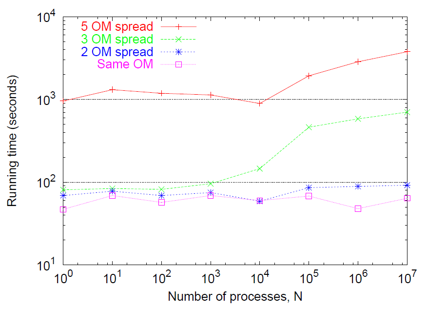
Figure 3: Performance of adaptive correction rejection method as a function of the number of parallel processes, \(N\). For low to moderate \(N\) and spreads the running time is roughly constant. Rates are sampled from log-normal distribution [exponential of normally-distributed deviates with mean zero and variance \(\sigma^2\)]. The spread is estimated to be the ratio of the 95th upper- versus lower-percentiles of the normal distributions, \(e^{+2\sigma}/e^{-2\sigma}=e^{+4\sigma}\). \(10^6\) events were simulated and on each event the associated rate was resampled.
Unfortunately, for large spreads the news is not as good: recall from Eq. 2 the expected number of trials grows as the ratio of the maximum rate over the average rate. If the rates are widely distributed then the highest may be orders of magnitude above average. In the tests this was simulated by setting \(\sigma\) large and Figure 3 demonstrates that this had a severe impact on performance (top curve) for all \(N\). So the efficiency of adaptive correction depends critically on the distribution of rates; ideally, it would be better to have a method that didn’t depend on the distribution (which may not be known in advance).
6. Roulette in a tree
— Rik Blok, 2004-10-14
I’ve thought of a faster way to implement the roulette wheel method. It relies on storing partial sums on a balanced binary tree structure and should run in \(O(\log_2 N)\) time, independent of the distribution of rates. Unlike the adaptive correction rejection method the rates are now explicitly stored and manipulated as part of the data structure and each process must be labelled by an index \(i=1,\ldots, N\) in order to access its corresponding rate.
The tree, shown in Figure 4, is important because it is guaranteed to be as well balanced as possible for any number of processes, \(N\). Further, it is easy to add or remove processes as necessary. (Removing is done by setting the appropriate rate to zero but leaving it in the tree.) Locating a node is also efficient, requiring \(O(\log_2 N)\) operations.
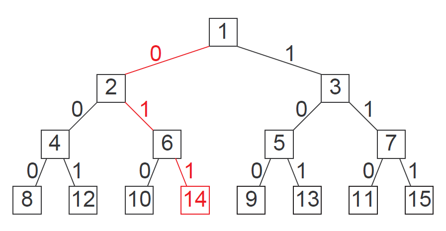
Figure 4: A binary tree with a one-to-one mapping onto positive integers. Each node has two children indicated by the branches 0 and 1. To locate the node representing an index we represent the index in binary. Starting at the root (which is always index 1) we follow the branches by reading the binary representation from right to left until we reach the final 1. For instance, the highlighted path to \(i=14\) (1110 in binary) is \(0\rightarrow 1 \rightarrow 1\).
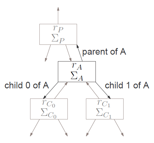
Figure 5: A single node in the binary tree used to optimize the roulette wheel algorithm. Each node \(A\) contains a rate \(r_A\), sum of rates \(\Sigma_A\), and links to its parent \(P\) and children \(C_0\) and \(C_1\). \(\Sigma_A\) is the sum of all the rates down the branch of \(A\), including \(r_A\) itself, \(\Sigma_A = r_A + \Sigma_{C_0} + \Sigma_{C_1}\). Any non-existant nodes are assumed to have \(r=\Sigma=0\).
But the real value of the binary tree is in how it “divides and conquers” the roulette wheel. We store in each node the rate of the associated process \(r_A\) and the sum of the rates in all nodes beneath it \(\Sigma_A\) as shown in Figure 5. Recall, in the roulette wheel we draw a single random number \(u\) between zero and the sum of all rates and then iterate through each process to determine which one \(u\) “landed” on. The binary tree reduces that process because we can determine in one comparison whether \(u\) landed on any processes along a branch. If it did, then we proceed down that branch and compare again, recursively, to find the node that \(u\) selects.
For a given node \(A\) (with children \(C_0\) and \(C_1\) as shown in Figure 5) and random \(u\) in \([0,\Sigma_A)\) there are three possibilities: if we line up the probabilities \(r_A\), \(\Sigma_{C_0}\), and \(\Sigma_{C_1}\) for the roulette wheel (see Figure 6) then \(u\) will land in the domain of \(r_A\) or \(\Sigma_{C_0}\) or \(\Sigma_{C_1}\). The algorithm to choose a random event follows:
- Start at root of tree, \(A=\text{root}\).
- If \(u < r_A\) then choose \(A\).
- Otherwise, \(u\gets u - r_A\) (so that \(u < \Sigma_{C_0} + \Sigma_{C_1}\)).
- If \(u < \Sigma_{C_0}\) then set focal node \(A=C_0\) and repeat from Step 1.
- Otherwise, set \(u\gets u - \Sigma_{C_0}\) (so that \(u < \Sigma_{C_1}\)), set focal node \(A=C_1\), and repeat from Step 1.
The full code is given in Listing 2.

Figure 6: To select an event via the binary tree Roulette Wheel algorithm pick a random number \(u\) between 0 and \(\Sigma_A = r_A + \Sigma_{C_0} + \Sigma_{C_1}\). The area it lands in indicates the course of action (choose \(A\) or branches \(C_0\) or \(C_1\), respectively).
class TPPNode {
// nodes for TParallelPoisson tree.  Each node uses ~32 bytes.
  private:
    TPPNode *odd;
    TPPNode *even;
  public:
    TPPNode *parent;
    unsigned long index;  // >= 1
    double rate;
    double sum;
    TPPNode(TPPNode *newparent = NULL, unsigned long path = 0x1) {
    // constructor
      parent = newparent;
      rate = sum = 0;
      odd = even= NULL;
      // reverse path to get index
      for (index = 1; path > 1; path = (path >> 1))
        index = (index << 1) | (path & 0x1);
    }
    ~TPPNode() {
    // destructor
      if (odd)  delete odd;
      if (even)  delete even;
    }
    TPPNode *getNode(unsigned long find, bool create,
                     unsigned long path = 0x1) {
    // returns pointer to node with index==find
    // creates node(s) if create==true,
    // else returns NULL if not found
      if (find == 1)  return this;
      path = path << 1;  // shift bits
      if (find & 0x1)  {
        path |= 0x1;  // append 1
        if (!odd) {
          if (!create)  return NULL;
          odd = new TPPNode(this, path);
        }
        return odd->getNode(find>>1, create, path);
      } else {
        if (!even) {
          if (!create)  return NULL;
          even = new TPPNode(this, path);
        }
        return even->getNode(find>>1, create, path);
      }
    }
    unsigned long choose(double roulette) {
      if (roulette < rate)  return index;
      roulette -= rate;  // now roulette < odd->sum + even->sum
      double oddsum = 0, evensum = 0;
      if (odd)  oddsum = odd->sum;
      if (even)  evensum= even->sum;
      if (roulette < oddsum)
        return odd->choose(roulette);
      return even->choose(roulette - oddsum);
    }
};

class TParallelPoisson {
/*
  Intended usage:

  // setup
  TParallelPoisson pp;
  unsigned long event;
  double time = 0;
  for (int i=1; i<=N; i++)
    pp.setRate(i,rate[i]);  // note: must be base 1!
  // main loop
  do {
    event = pp.choose(uniform_deviate());
    time += pp.eventTime(uniform_deviate());
    do_stuff(event);
    for (EACH_RATE_CHANGED_BY_EVENT) {
      pp.setRate(i,rate[i]);
    }
  } while (!HELL_FROZEN_OVER);
*/
  private:
    TPPNode *root;
  public:
    TParallelPoisson() {  // constructor
      root = new TPPNode;
    }
    ~TParallelPoisson() {  // destructor
      if (root)  delete root;
      root = NULL;
    }
    void reset() {
      if (root)  delete root;
      root = NULL;
      root = new TPPNode;
    }
    double eventTime(double u) {
    // returns time to first event.  Assumes 0 <= u < 1.
      if (!root)      return 0;
      if (!(root->sum))  return 0;
      return -log(1.0-u)/(root->sum);
    }
    double getRate(unsigned long i) {
    // gets rate of node i (zero if not found)
      TPPNode *node=root->getNode(i,false); // don't create node
      if (!node)  return 0;
      return node->rate;
    }
    double setRate(unsigned long i, double newrate) {
    // sets rate of node i, returns old rate
      TPPNode *node=root->getNode(i,true); // create node if needed
      double oldrate = node->rate;
      double dr = newrate - oldrate;
      node->rate = newrate;
      for (; node; node = node->parent)  node->sum += dr;
      return oldrate;
    }
    double modRate(unsigned long i, double deltarate) {
    // adjust rate of node i, returns new rate
      TPPNode *node=root->getNode(i,true); // create node if needed
      double newrate = node->rate + deltarate;
      node->rate = newrate;
      for (; node; node = node->parent)  node->sum += deltarate;
      return newrate;
    }
    unsigned long choose(double u) {
    // chooses which event happens next, assumes 0 <= u < 1
      if (!root)  return 0;  // error value
      if (!(root->sum))  return 0;  // error value
      return root->choose(u * root->sum);
    }
};
Listing 2: C++ implementation of binary tree roulette wheel method.
7. References
- Blok (2004)
- Blok, H.(2004, 10/15). Retrieved from https://www.cs.ubc.ca/~rikblok/research/notes/parallel_poisson/index.html